|
Determining Query Performance Metrics
The performance of an application can be influenced by many things. Hardware constraints such as lack of memory or slow disk sub system can be just as detrimental as application inefficiency. However, in many situations the first is caused by second. An inefficient application can be cheaper and easier to fix in the long run, then creating server farms or buying huge, super-beefy equipment and paying lots of people to keep it up and running. (Not to mention increasing the payment for the electric bill, insurance, network infrastructure, power supplies, etc.)
Analysts will tell you that the cheapest way to solve application problems is to start when you are designing the system. “Design for efficiency” they’d say, and they’d be right. (They’d better be for the amount of money we pay them.) However, many of us in “real world” don’t always have the luxury of being able to do this. In many cases, the design of the system is already set when we come on board and we aren’t allowed to influence it much.
The key to improving performance of any application that is already written and working in production is to identify the problem areas and target your changes for the areas that will either have the biggest improvement for the users, or that will make the fewest requests of the hardware. In a database application, it is usually best to start with the database and work your way out from there to application servers, or web servers. This is because no matter how many layers or tiers you have in an application, if the database is not performing well, the entire application suffers. Sure this can be masked with caching and such, but most of the common performance problems start with the database.
SQL Server comes with many tools to allow you to identify performance issues. SQL Profiler is a great tool for tracing what is going on for a period of time. SQL Server 2005 has a built in scheduled trace that captures performance information about queries running in the system, but that might not be enough for your situation. If it isn’t, one could schedule their own trace looking for queries that run longer than a certain time, for example, in order to get more information.
Session Blocking can also impact performance. Blocking is caused when two different SQL sessions try to access the same piece of data at the same time and place a lock on the data. When Session “A” has a lock on the data and Session “B” tries to place a lock on the same piece of data, Session “B” must wait until Session “A” releases its lock. This is one of the more common “phantom slowness” problems experienced with applications. The application runs fine normally but every now and then, it is just as slow as molasses. This situation can be detected by querying the “sysprocesses” table. In fact, it is highly recommended that systems that are experiencing performance issues have a scheduled job that captures the “blocked<>0” rows into a logging table so that any database blocking can be identified during and after the fact and patterns can be established.
The following query can identify the Session “B” connections that are being slowed down by the blocking sessions.
Select A.*
From dbo.sysprocesses as A with (nolock)
Where A.blocked <> 0
And A.blocked <> A.spid
The following query can identify the Session “A” connections that are the root cause of the blocking. This could be something like a backup job, a DBCC command, or just a general query in the system.
Select A.*
From dbo.sysprocesses as A with (nolock)
Where A.blocked = 0
And A.spid in (Select B.blocked
From dbo.sysprocesses as B with (nolock)
Where B.blocked <> 0
And B.blocked <> B.spid)
Blocking can be alleviated by using a SQL Server 2005 setting for a database connection called “Snapshot Isolation”. It is a type of transaction isolation level that will allow simultaneous reads of a particular piece of data even while the data is being written to. This method will increase the usage of the TempDB database so be wary of this when using it. One can also decrease blocking by strategically using NOLOCK query hints in places where one can get away with it. Use proper testing and QA techniques to identify if any changes such as these impact the performance of an application negatively before implementing.
Regardless of which method identifies a bad performing query, once you have found it, what do you do about it? “I have this bad query, which gives me the data I want, but runs slow… can you fix it?” This is a common question asked of DBAs by developers. Many developers can make application do ultra snazzy, fancy things, but are not savvy when it comes to query optimization.
The rest of this article is dedicated to trying to go through the process of identifying the slow parts of a query, and ways of computing which areas are the slow areas of the query.
1) Generate a Query Plan
There are several ways within SQL Server Management Studio to do this. The easiest way is to have your query open in a query window and click the “Display Estimated Execution Plan” button located on the toolbar that looks like the following icon: 
We’ve generated an extremely inefficient table with 1,000,000 rows of data in it in order to illustrate costs of doing various types of optimizations in order to show the impact of our changes. Consider the following query in the sample database.
SELECT A.SmallDateFlag,
B.DateTimeFlag
FROM PerfExample.dbo.TransactionTable1 as A
Left Outer Join PerfExample.dbo.TransactionTable1 as B
on (A.TransactionID = B.TransactionID and B.CharFlag = 'Y')
Where A.CharFlag = 'B'
This will show you something like the following example plan.
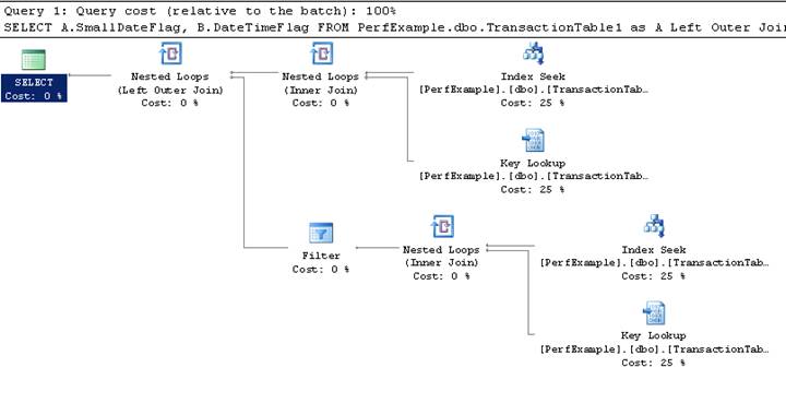
In order to determine the order that things execute in a query plan you have to read it right to left, top to bottom, for each branch.
For a complete list of what these icons mean and how each one works, visit the following web address.
http://msdn2.microsoft.com/en-us/library/ms175913.aspx
So, the first thing that executes is an “Index Seek”. An index seek is going to use a non clustered index to more rapidly look up data in a table than and “row by row” loop (called a scan) through the table. This is one of the more efficient methods of finding data within a database.
The next thing is a “Nested Loop Inner Join”, but that is tied to a “Key Lookup” operation. So, a simple way to interpret this logically is that for each row found in the “index seek”, a “key lookup” operation will be performed. A key lookup is an operation that looks up the actual row in the physical table that corresponds to the row found in the index seek. There is also a related step called “Bookmark Lookup” (not shown in this plan) that is similar to a “Key Lookup”. The difference is that in a table with a clustered index, rows can be more efficiently stored in the database and can be retrieved by using the keys found in the clustered index. However, tables that do not contain clustered indexes (also referred to as Heap tables) must use a more physical addressing method to retrieve the data from the table once it is found with an index.
Please use the article references to walk through the plan shown, or any of your own query plans, until you are comfortable with the different icons and terms and what they mean.
2) Determine the Cost of a Query
Once a plan has been calculated and displayed, there are some steps one can follow to determine the cost of the query.
The cost of any piece of a query can be determined by highlighting the step in the plan and then hovering over it with your mouse. The cost of the entire query can be found by going to the “select” step (which can also be Insert/Update/Delete or any number of things, but these are most common, and are usually the left most item on the query plan.
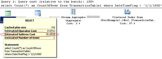
In this example, the left most step in the query, which was the “select” part of the SQL batch, shows an amount of 35.8529 as the “Estimated Subtree Cost”. Subtree Cost means the cost of this step as well as all of the steps that came before this one all added together. So in this case, the subtree cost is for the whole query, whereas it could just as easily been a piece of the query to tell you the cost from that point to the beginning.
Query Cost amounts are not in direct correlation to a time. They are a cost estimate of how much “effort” must be put forth to execute the query.
SQL Server uses what is called a Query Optimizer to determine the best overall method of executing each query. SQL Server’s query optimizer uses a “Cost Based” method for determining the best plan or method for query execution. The cost value calculated by the query optimizer is based upon several factors related to the query.
The following is a simplistic list of possible things that the optimizer would look at. How much of the CPU will the query use? Are there lots of computations to perform in this query? Are the values for the columns in the where clause estimated to be found a great deal in the table or are they fairly unique? (To determine this, SQL Server uses database Statistics) How many estimated disk requests must the server make to fulfill this request? Are there better access paths toward finding the data (indexes) or do I need to loop through all of the data to find what I’m looking for (scan)? These and many other things can be evaluated when a query is executed in order to figure out how costly a query is. When finished, the optimizer chooses what it computes is the best execution plan for gathering the data in the most efficient way. Then overall cost of each step can be aggregated up to a single number… the overall query cost.
This overall cost can be used as a benchmark for query performance; however, it can be misrepresenting. Some feel that a better benchmark is to use the CPU and IO associated with a query to determine how many computations and reads/writes a query will perform. This is a factor which will stay relatively the same between a test server and a production server, but the cost could be radically different. All of these metrics, however, are to be used together to form the overall effort required to execute a query.
3) Determine the CPU and Disk I/O Used to Execute a Query
Finding out the amount of CPU time and Disk Reads/Writes (I/O) are being requested for a given query is a fairly simple process. There are two commands that one can execute, prior to running a query, that will give this information within the messages window of SQL Server Management Studio.
SET STATISTICS IO ON;
SET STATISTICS TIME ON;
The “Statistics IO” session setting tells SQL Server to output the amount of Logical and Physical Reads and Writes were performed while executing a query. Physical Reads and Writes refer to reads and writes that must be made to the physical disk subsystem and not to the data cache which is stored in RAM. SQL Server will automatically store commonly referenced data pages in memory for faster access. When SQL Server is making a request to Read or Write to these cached pages, these are referred to as Logical Reads and Writes. A read or write is taking place, but these are much faster than hitting the disk sub system. However, since there is little control over which data pages are stored in the cache, and since 300GB databases cannot be totally stored in Memory on almost any affordable server, Physical disk access will occur. The goal is to limit the total amount of reads and/or writes a query must perform in order to reduce the amount of resources (memory or disk) are requested.
The “Statistics Time” session setting tells SQL Server to output two different execution time and CPU values. The first one is displayed before the execution of the query begins. This is the amount of time and number of CPU milliseconds required to calculate the cost and
of a query. This happens for every query regardless of whether or not it is already parsed; however, if a query is already in the procedure cache and already has a cost and plan calculated, these values will be low if not zero. In that case, it is the time that it took to find the query in the procedure cache. Whenever you execute a query multiple times, it will show a smaller value for the first number on subsequent executions (assuming no change has been made to the query) so be mindful of this. The second value for the execution time and CPU time refer to the time that it actually took to execute the query.
Why would anyone need to know how long a query took to compile versus how much time to execute? There are times on complicated queries with lots of computations, or queries that use tables with out of data statistics, where the time to calculate the query plan actually takes longer than the actual execution of the query. By looking at both values, those cases can be identified as well.
Here is an example of this in action. Consider the following query similar to the one from before.
SELECT A.SmallDateFlag,
B.DateTimeFlag
FROM PerfExample.dbo.TransactionTable1 as A
Left Outer Join PerfExample.dbo.TransactionTable1 as B on (A.TransactionID = B.TransactionID and B.CharFlag = 'Y')
Where A.CharFlag = 'Y'
By setting these options, we can see the following results in the Messages window.
SQL Server parse and compile time:
CPU time = 16 ms, elapsed time = 220 ms.
(1000000 row(s) affected)
Table 'Worktable'. Scan count 0, logical reads 0, physical reads 0, read-ahead reads 0, lob logical reads 0, lob physical reads 0, lob read-ahead reads 0.
Table 'TransactionTable1'. Scan count 2, logical reads 91248, physical reads 0, read-ahead reads 17717, lob logical reads 0, lob physical reads 0, lob read-ahead reads 0.
SQL Server Execution Times:
CPU time = 2531 ms, elapsed time = 107810 ms.
As you can see from the different times and values, this query took 16 milliseconds of CPU time and 220 milliseconds to compile. It took 2.5 seconds of CPU time to execute and 107 seconds to execute. The TranstionTable1 table had to be scanned twice. The logical number of reads was 91,248 and the read-ahead reads (which are the number of physical reads that occurred to populate the data cache with data for this query) was 17,717. This brings the total number of data pages read up to 108,965. Each data page read was 8K a piece, so the total number of bytes read for this query was 892,641,280 bytes or 851MB. That may not seem too bad, but let’s consider if this query were a transaction query for a major retail application. Let’s say that it had to read 851MB every time a customer “checked out” of a sale and this site had a goal of processing 1,000 orders a day. Now the disks and memory need to be able to process 810 gigabytes of data per day to meet that goal, just to execute this one query, not to mention everything else that the system would need to do. So, one can see quickly that a really inefficient query in the wrong place can put great strains on the hardware.
Conclusion
There are many situations in which the effort that equipment has to go through to fulfill the needs of an application is unknown. However, as Francis Bacon (inventor of the “Scientific Method” for investigating scientific phenomenon and gathering empirical evidence to support findings) once said, “Knowledge is Power”. If one has the knowledge to discover which pieces of their system is performing slower, and the knowledge to be able to quantify how slow something is, then they will have the power to resolve the issue. Hopefully, this article has given some helpful tips for you to be able to calculate the resources consumed by queries, thereby giving you the ability to prioritize which queries will benefit the most from the development effort of optimization.
|